Monday: Today I put all the data from our RTD excel document into Matlab and we ended up getting the same graph. I saw feature in Matlab that gave us the option of changing the amount of significant figures. When I did this, we got much better results that fit Dr. Ramachandran's criteria. Other than that, we didn't really do much today.
Tuesday: Today Dr. Ramachandran asked us to find out a couple more things regarding the RTD. He wanted us to actually plot the RTD graph which is modeled by the equation where E(t) is the residence time distribution and C(t) is our concentration as a function of time. Dr. Panikar forgot some of her calculus because she is more involved in experimental work. So she asked me to do this part of the analysis. Because our concentration function is not modeled by an actual expression, I had to use a Riemann sum estimate. I used a right Riemann sum with each section being a rectangle. This gave me the denominator of the function. We already have our C(t) values which were obtained a while ago and now we just had to plot E(t) for every C(t) value. Dr. Ramachandran also wanted us to find out the Mean Residence Time (MRT) which is modeled by the equation
 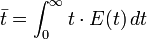 where tau is the MRT, t is time, and E(t) is our residence time distribution. Again I had to use a Riemann sum to evaluate the integral because we don't have an equation for our E(t) function. So first, I multiplied each time by the E(t) value and got t*E(t). Since dt is just a differential, I could substitute it for my delta t which is just 10 (Riemann Sum interval). So this is equal to t*E(t)*10. To find tau, you just add all of these values up for each time and you get your MRT. We were required to find the mean centered variance (MCV) which is modeled by the equation
 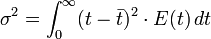 where o^2 is equal to the MCV, t is equal to time, tau is equal to MRT, and E(t) is equal to the RTD. What I did to solve this equation is first I evaluated the expression that was inside the integral excluding dt for each time value that we had. Then I replaced dt with 10, our interval size, and multiplied each value by 10. Lastly, I added all of these values up and got the MCV. Dr. Ramachandran asked us to find the standard deviation which is just the square root of the MCV. I did this for our 4 trials. The last thing Dr. Ramachandran wanted us to do was to take the integral of the % concentration graph (C(t)) and find out how much dye was injected at the start of each trial. Dr. Panikar and I had trouble with this because we didn't know what the units of the integral should be. We were integrating % concentration but we didn't know what units the % concentration were in. We are still working on this and trying to find the solution.
Wednesday: Today we finally found out what the units of the integral of the concentration curve was. First of all, in order to find out the amount of dye that is injected at the start of the RTD, you have to use this equation: where N0 is the mass of the tracer, v is the volumetric flow rate of the feeder, and C(t) is the concentration of dye from the exit stream. The volumetric flow rate of our feeder is 35 grams/minute. However, we have to convert it into grams per seconds because our time on our concentration graph is in seconds. Then you get 7 grams/12 seconds. Now it got tricky when we tried to think about the units for % dyed or the concentration function. What units does % dyed have? We backtracked to our calibration samples and the machine measured the % dyed using mass. For example, 50% of the sample is dyed when there are 50 grams of dyed sample and 50 grams of undyed sample. So the % dyed is just grams/grams which is basically dimentionless. So we ended up getting grams as our units for the amount of tracer. We also started working on the NIR project. I will explain this in more detail in Thursday's section.
Thursday: Today I started editing the powerpoint to make it more sophisticated because Dr. Panikar has a tele-conference on August 12th and she will need a powerpoint to present the results. She wants the powerpoint done before I am gone because she has another conference from August 2-10th. So I put in the calculation results that we got yesterday and described how they related to the experiment. In the muller, the powder is perfectly mixed if the MCV is equal to 1. We had one trial with a MCV of 0.94 which is very good. I also added the E(t) graphs and explained how they related to the concentration graphs. I had to read some papers on RTD to get a more complete understanding of what RTD really is. However, these papers assumed that everyone already knows what RTD really is. Instead, they consisted of relationships between RTD and other properties of the mixing and particles. Dr. Panikar did not come in today because something unexpected came up. She told me to work on this powerpoint and the NIR. The entire NIR project is very different than the RTD project; in fact they are 2 separate projects. The NIR is used to characterized the product that we get from the muller when the powder and water are mixed together. We ran this kind of experiment during my first few days in the lab. I'm still not sure what exactly the NIR measures but it seems very important because it is used a lot not only in my project but in other projects. What we are doing now is trying to find a way for the NIR to sense the paste that comes out of the muller. When the paste comes out of the muller, it comes out in a very sporadic, irregular way. So the NIR will be taking pictures of mostly air and then the paste. Dr. Panikar doesn't want the NIR to be taking pictures of the air because then she will have to go through the files and delete them manually which makes the process longer. So she is trying to engineer a way for the paste to be collected somewhere and then the NIR could take a picture of it. She explained a way for us to do this but I can't really explain it in words only so I'll try to get a picture of it. But all of those materials are dirty so she also told me to clean them if I have the time after finishing the powerpoint. I was able to clean the materials and by the time I was done with all of this, it was 2:30 p.m. This was awesome because recently I have been working in the lab until 6:00 so today I was able to leave early. And best of all, there was no traffic on the roads.
Friday: Today was a very short day because we didn't have the feeder to conduct some of our experiments. We actually borrowed the feeder from one of Dr. Ramachandran's other projects and they ended up needing it. So we won't be able to do any experiments until they are done with the feeder which will probably be next Wednesday. For now, we are planning our setup for the experiments and how we are going to conduct them. These experiments include running the RTD and seeing how the muller RPM and feeder rate will affect the residence time. Also, we presented our results to Dr. Ramachandran and he was pleased with them. He told us that we only had to do the powder dye method instead of the liquid dye method because clearly, the results indicate that the liquid dye method is not good. Also, Dr. Ramachandran said that he would write a recommendation for me so I was pretty happy about that.
Tuesday: Today Dr. Ramachandran asked us to find out a couple more things regarding the RTD. He wanted us to actually plot the RTD graph which is modeled by the equation
where E(t) is the residence time distribution and C(t) is our concentration as a function of time. Dr. Panikar forgot some of her calculus because she is more involved in experimental work. So she asked me to do this part of the analysis. Because our concentration function is not modeled by an actual expression, I had to use a Riemann sum estimate. I used a right Riemann sum with each section being a rectangle. This gave me the denominator of the function. We already have our C(t) values which were obtained a while ago and now we just had to plot E(t) for every C(t) value. Dr. Ramachandran also wanted us to find out the Mean Residence Time (MRT) which is modeled by the equation where tau is the MRT, t is time, and E(t) is our residence time distribution. Again I had to use a Riemann sum to evaluate the integral because we don't have an equation for our E(t) function. So first, I multiplied each time by the E(t) value and got t*E(t). Since dt is just a differential, I could substitute it for my delta t which is just 10 (Riemann Sum interval). So this is equal to t*E(t)*10. To find tau, you just add all of these values up for each time and you get your MRT. We were required to find the mean centered variance (MCV) which is modeled by the equation where o^2 is equal to the MCV, t is equal to time, tau is equal to MRT, and E(t) is equal to the RTD. What I did to solve this equation is first I evaluated the expression that was inside the integral excluding dt for each time value that we had. Then I replaced dt with 10, our interval size, and multiplied each value by 10. Lastly, I added all of these values up and got the MCV. Dr. Ramachandran asked us to find the standard deviation which is just the square root of the MCV. I did this for our 4 trials. The last thing Dr. Ramachandran wanted us to do was to take the integral of the % concentration graph (C(t)) and find out how much dye was injected at the start of each trial. Dr. Panikar and I had trouble with this because we didn't know what the units of the integral should be. We were integrating % concentration but we didn't know what units the % concentration were in. We are still working on this and trying to find the solution.Wednesday: Today we finally found out what the units of the integral of the concentration curve was. First of all, in order to find out the amount of dye that is injected at the start of the RTD, you have to use this equation:
where N0 is the mass of the tracer, v is the volumetric flow rate of the feeder, and C(t) is the concentration of dye from the exit stream. The volumetric flow rate of our feeder is 35 grams/minute. However, we have to convert it into grams per seconds because our time on our concentration graph is in seconds. Then you get 7 grams/12 seconds. Now it got tricky when we tried to think about the units for % dyed or the concentration function. What units does % dyed have? We backtracked to our calibration samples and the machine measured the % dyed using mass. For example, 50% of the sample is dyed when there are 50 grams of dyed sample and 50 grams of undyed sample. So the % dyed is just grams/grams which is basically dimentionless. So we ended up getting grams as our units for the amount of tracer. We also started working on the NIR project. I will explain this in more detail in Thursday's section.Thursday: Today I started editing the powerpoint to make it more sophisticated because Dr. Panikar has a tele-conference on August 12th and she will need a powerpoint to present the results. She wants the powerpoint done before I am gone because she has another conference from August 2-10th. So I put in the calculation results that we got yesterday and described how they related to the experiment. In the muller, the powder is perfectly mixed if the MCV is equal to 1. We had one trial with a MCV of 0.94 which is very good. I also added the E(t) graphs and explained how they related to the concentration graphs. I had to read some papers on RTD to get a more complete understanding of what RTD really is. However, these papers assumed that everyone already knows what RTD really is. Instead, they consisted of relationships between RTD and other properties of the mixing and particles. Dr. Panikar did not come in today because something unexpected came up. She told me to work on this powerpoint and the NIR. The entire NIR project is very different than the RTD project; in fact they are 2 separate projects. The NIR is used to characterized the product that we get from the muller when the powder and water are mixed together. We ran this kind of experiment during my first few days in the lab. I'm still not sure what exactly the NIR measures but it seems very important because it is used a lot not only in my project but in other projects. What we are doing now is trying to find a way for the NIR to sense the paste that comes out of the muller. When the paste comes out of the muller, it comes out in a very sporadic, irregular way. So the NIR will be taking pictures of mostly air and then the paste. Dr. Panikar doesn't want the NIR to be taking pictures of the air because then she will have to go through the files and delete them manually which makes the process longer. So she is trying to engineer a way for the paste to be collected somewhere and then the NIR could take a picture of it. She explained a way for us to do this but I can't really explain it in words only so I'll try to get a picture of it. But all of those materials are dirty so she also told me to clean them if I have the time after finishing the powerpoint. I was able to clean the materials and by the time I was done with all of this, it was 2:30 p.m. This was awesome because recently I have been working in the lab until 6:00 so today I was able to leave early. And best of all, there was no traffic on the roads.
Friday: Today was a very short day because we didn't have the feeder to conduct some of our experiments. We actually borrowed the feeder from one of Dr. Ramachandran's other projects and they ended up needing it. So we won't be able to do any experiments until they are done with the feeder which will probably be next Wednesday. For now, we are planning our setup for the experiments and how we are going to conduct them. These experiments include running the RTD and seeing how the muller RPM and feeder rate will affect the residence time. Also, we presented our results to Dr. Ramachandran and he was pleased with them. He told us that we only had to do the powder dye method instead of the liquid dye method because clearly, the results indicate that the liquid dye method is not good. Also, Dr. Ramachandran said that he would write a recommendation for me so I was pretty happy about that.
No comments:
Post a Comment